GEOG 338: Lab 6

Lab 6: Geometric Correction

Melissa Hackenmueller

Background

Lab six was designed to introduce students to geometric correction. Geometric correction is very important in image pre-processing for it needs to be used to accurately extract biophysical and sociocultural information. Two types of geometric corrections will be performed in this lab. The first is image-to-map rectification and the second is image-to-image rectification.

Methodology

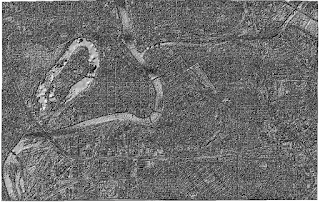
            The first section of this lab uses a USGS 7.5 minute digital raster graphic image of the Chicago Metropolitan Area and a corrected Landsat TM image of the same area. The first step is to input both the Chicago_drg.img and the Chicago_2000.img into Erdas Imagine. Next, I clicked on the control points tool of the multispectral toolbox. A select geometric model dialog will open. I selected polynomial, then image layer, added my reference map (Chicago_drg.img), and then hit okay one last time in the reference map information dialog. This then will bring up a multipoint geometric correction window. This window showed my input image (Chicago_2000.img) on the left and my reference image (Chicago_drg.img) on the right. Ground control points could now be added to my maps, but I first made sure that any existing ground control points were deleted. Then I used the create ground control points tool to input a point on each map in the same area. I then repeated this process three more times to get four ground control points that were evenly distributed across my images. Once, this was done I looked at my total RMS error and it was very high. To decrease the RMS error, I zoomed into each ground control point and adjusted it to accurately represent the area on the other image. Once my RMS error was below 2 I decided that my image was spatially correct enough for this project (Figure 1). Ideally the RMS error should be below 0.5 for the geometric correction to be accepted in the remote sensing field. I was content with my RMS error so I used the display resample dialog button to create a rectified, geometrically correct image.

            Part two of this lab was to use image-to-image rectification to create a geometrically correct image of the east side of the Sierra Leaone. I started by importing the sierra_leone_east1991.img and the sl_reference_image.img into two separate viewers in Erdas Imagine. I then chose control points from the multispectral toolbar. In the geometric model window I selected polynomial, then image layer, imported my reference map (sl_reference_image.img), accepted the default inputs for the reference map information, and finally chose 3^rd order polynomial. I then clicked on the create ground control points tool and started to add my points as I did in part one. This time I added 12 ground control points to my image. Only 10 are needed for 3^rd order polynomial, but a few extra points allow the rectification to be more accurate. Once I placed all my ground control points, I more accurately placed them until my RMS error was below 1 (0.5 would be ideal, but was not necessary for this lab). Figure 2 is an image of my RMS error. I was content with my RMS error so I used the display resample image dialog button to create a geometrically correct image (sl_east_gcc.img). This image could then be used to more accurately analysis the area of interest.

Results

Figure 1: This image displays the ground control points that I used for my image-to-map rectification.
The ground control points are distributed evenly about the image to provide an accurate output image.
My RMS error is below 2, which was the goal for part one of this lab.

Figure 2: This image displays my ground control points for my image-to-image rectification. 

The RMS error is below 1 as that was the goal for part two of this lab. 

References

Satellite images are from Earth Resources Observation and Science Center, United States Geological Survey.

Digital raster graphic (DRG) is from Illinois Geospatial Data Clearing House.

GEOG 338: Lab 5

Lab 5: Lidar Remote Sensing
Melissa Hackenmueller

Goals & Background

            The primary objective of Lab 5 was to learn the basics of lidar data structure and processing. In order to obtain these goals, the lab was separated into three parts. The first of which was an introduction to point cloud visualization in Erdas Imagine in comparison to ArcMap. The second portion of this lab was created to learn how to generate a LAS dataset and gain experience with lidar point clouds on ArcGIS. The last section of this lab was designed to give students an introduction to the generation of lidar derivative products (DSM, DTM, and intensity images).

Methodology

            Part one of this lab uses Erdas Imagine and ArcMap to display lidar point cloud data. The first step I conducted was selecting all the LAS files of interest into Erdas Imagine. Next, I opened the tile index file QuarterSections_1.shp into ArcMap to locate my LAS data in Erdas Imagine. In doing this, I learned that ArcMap is much easier to analysis lidar point cloud data from than Erdas Imagine. Therefore, part two and three will be mainly using ArcGIS systems instead of Erdas Imagine.

            The objective of part two was to generate a LAS dataset and then explore the data within ArcMap. The first step was to add a new LAS dataset in ArcMap; I named mine Eau_Claire_City to give a description of what the study area is about. Next, I went to the LAS Dataset Properties of my newly made dataset and added all the LAS files needed from my project. After this I went to the statistics tab of the properties and hit calculate to produce statistics for the data I just imported. Statistics for the entire dataset will populate and statistics for individual files can be found on the LAS file tab. I then used these statistics to do a QA/QC check by comparing my minimum Z and maximum Z values with the known elevation of my study area, in this case, Eau Claire. The next step is to add coordinate systems to your dataset. After consulting the metadata, I determined that the NAD 1983 HARN Wisconsin CRS Eau Claire (US Feet) projection was the best fit for my XY coordinate system. I learned from the metadata that the NAVD 1988 US feet projection should be used for the vertical coordinate system of this data. This then concluded the editing of the new dataset, so I added the Eau_Claire_City.lasd into ArcMap to display it. I then added a shapefile of Eau Claire county to confirm that my dataset was properly located; it was and so I then removed the county shapefile (Figure 1). Next, I zoomed into my a small portion of my dataset to analyze my point cloud data (to save time the data doesn’t load the point cloud data at full extent). Once, zoomed in your data should appear, similar to Figure 2. Next, I used the LAS Dataset toolbar to examine the aspect, slope, and contours of my dataset. Another tool I utilized on the LAS Dataset toolbar was the profile view tool, this allows you to draw over a portion of interest on the map and then display a cross-sectional view of the point cloud data. This data can be viewed in 2D and 3D. Now, that I have my LAS dataset created in ArcMap, it is time to create products from it.

Figure 1: My LAS dataset lies correctly within the Eau Claire County shapefile confirming that the properties of my Eau_Claire_City LAS dataset were properly imputed. 

Figure 2: This shows a small portion of my point cloud dataset. The dataset must be zoomed in to in order for the point cloud data to display. 

             The objective of part three was to take the Eau_Claire_City LAS dataset and generate various lidar derivative products. First, I created a DSM using the LAS dataset to raster tool. My input was the LAS dataset and I named my output EC_FR_2m. I then chose the binning method and imputed the value field to elevation, the cell type to maximum, the void filling to Natural_Neighbor, the sampling type to Cellsize, and the Sampling Value field to 6.56168 ft (roughly 2 m). After these inputs were completed I ran the tool. To enhance the DSM that I just created I used the Hillshade tool from the 3D analyst tools. I imported the EC_FR_2m file I just created and ran the tool. Figure 3 is the hillshade DSM product that I created. My next goal was to create a DTM derivative. I made sure that my filter on the LAS Dataset toolbar was set to ground and the point tool to elevation. I then used the LAS dataset to raster tool again. I named the DTM, EC_DTM_2M and used all the same binning method parameters as before, except I chose minimum as the cell assignment type. I ran the tool creating my DTM and then I used EC_DTM_2M file to create a hillshade image. Figure 4 shows the bare earth product that I created in this step. The final derivative product that I created in this lab was a lidar intensity image. First, I set my dataset to point and the filter to first return. I then opened the LAS dataset to raster tool and imported the Eau_Claire_City dataset into the input. I imputed Intensity into the value field, Average into the binning cell assignment type, Natural_Neighbor into the void fill, 6.56168 into the cell size, and named the output EC_Int. I ran the tool and the intensity image was added to the map. The contrast of the intensity map is difficult to see in ArcMap, so I imported the EC_Int.tiff file into Erdas Imagine to enhance the contrast (Figure 5).

Results 

Figure 3: The hillshade DSM derivative product that I created from my Eau Claire City point cloud data. 

Figure 4: The hillshade DTM (bare earth) derivative product that I created from the Eau Claire City point cloud data.

Figure 5: The Intensity image that I created from the Eau Claire City lidar point cloud dataset, displayed in Erdas Imagine. 

References

Lidar point cloud and Tile Index are from Eau Claire County, 2013. 

Eau Claire County Shapefile is from Mastering ArcGIS 6th Edition data by Margaret Price, 2014.

Geog 337: Lab 2

Lab 2: Watershed Analysis

Melissa Hackenmueller

Goal

The watershed analysis lab had two main goals. The first was to use ArcGIS to understand and master the skills needed to delineate watersheds of a specified region. The second goal was explore ModelBuilder and gain knowledge on the structure of workflows and its uses. 

Methodology

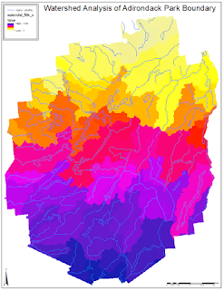
Part 1 was the delineation of watersheds. A watershed is an area of land that all surface water drains through a specific point (stream or lake) in that basin. All water within the watershed is connect; therefore, contamination in the upstream portion of a watershed will affect all of the downstream water. Therefore, the studying and understanding of watersheds is very important for environmental restoration and protection. This lab will delineate the watersheds of Adirondack Park in northeastern New York. The data for this lab was collected from the New York State GIS Clearinghouse and Cornell University's Geospatial Information Repository site. The first step of this project was to create a geodatabase and save both files in this newly formed geodatabase. The next step is processing the data. The projections for each of these files is different, so I used the data management tools to make sure the data was in a uniform projection coordinate system, which in this case was UTM Zone 18N NAD 1983 meters. Next, I created a 20 km buffer around the park boundary to create smoother watersheds later.  The clipping tool was used next to create a shapefile of just streams with Adirondack Park. A 30 arc-second DEM of North America was then added and converted to the correct coordinate system. I then clipped the DEM as well to fit the size of the buffered park boundary. The next step was to resample the data to a 60 m pixel size by using Project Raster in the Data Management tools. Now, the flow direction needs to be calculated using the flow direction tool from the Spatial Analysis Toolbox. I then found that sinks appeared in this data, which needed to be removed. I used the fill tool to do so, then did the process of flow direction again using the new filled file. Next, I used the flow accumulation tool to determine where flow accumulates. The Conditional tool was then used with a value of  >50,000 to show faint stream channels. I then created a source raster that showed unique stream links. Finally, the data was ready to use the watershed feature. Using the flow direction raster and the source raster as input, a watershed raster was created. Figure 1 shows the watershed delineation and the streams of Adirondack Park, New York. 

Part 2 was using ModelBuilder to find areas in Denmark at risk of flooding in a Cloudburst. Cloudbursts are sudden, extreme rainfall events that occur in a very short amount of time and overwhelm infrastructure and create major flooding. Using ModelBuilder a model can be built to find depressions in a specified region and building that overlap with those depressions; therefore, find the buildings at risk. A model was already created as an ESRI lesson and this is what I used to expand my knowledge of ModelBuilder and its uses. The first step was to locate the first model in the geodatabase and assess all of its properties. Then I validated and ran the model. This model then created new shapefiles of Bluespots (depressions in the landscape that are susceptible to flooding) and of Buildings touching bluespots. I added these new shapefiles to ArcMap and corrected the symbology and created Figure 2. Another model was then used to create a more in-depth map that included the volume and the watershed of the bluespots, as well as, the amount of rainfall needed to fill each bluespot. I ran this model and then corrected the symobology again to create Figure 3. Next, I added the watershed layer with discrete color symbology to correlate the bluespots and watersheds (Figure 4). 

Results

Figure 1

Figure 2

Figure 3

Figure 4

References

New York State GIS Clearinghouse. Adirondack Park Boundary Shapefile. http://gis.ny.gov/.

Cornell University Geospatial Information Repository. Hydrology Features of New York State. NatlAtlas. http://cugir.mannlib.cornell.edu/index.jsp. 

ERSI. Find Areas at Risk of Flooding in a cloudburst. https://learn.arcgis.com.