Geospatial Labs: GIS I, GIS II, and Remote Sensing: Geog 338: Lab 8

Spectral Signature Analysis and Resource Monitoring

Melissa Hackenmueller

Background and Goals

The main goal of this lab is to become more familiar with and gain hands on experience with the measurement and interpretation of spectral reflectance signatures. Part one of this lab will teach how to collect spectral signatures from satellite imagery, graph these signatures, and then analysis them. The second portion of the lab will be learning how to use Erdas Imagine to monitor the health of vegetation and soils using simple band ratio techniques. This will include mapping the findings using ArcMap.

Methodology

Part 1: Spectral Signature Analysis

I used a Landsat ETM+ image of Eau Claire and Chippewa counties, Wisconsin, to analysis the spectral signatures of 12 natural and man-made features. I first loaded the eau_claire_2000.img into Erdas Imagine. I then zoomed into a water feature called Lake Wissota to collect my first spectral signature. By using the polygon tool from the drawing tab, I digitized a small polygon within Lake Wissota. Then from the raster tools I selected supervised and then signature editor. The signature editor dialog is now open. I then created a new signature form AOI, which added a new row in the dialog box. I then changed the signature name to standing water, to ensure I would remember what each new signature represented. I then clicked on the display mean plot window tool to display the plot of the spectral signature (Figure 1). I then followed the same process above with moving water, deciduous forest, evergreen forest, riparian vegetation, crops, dry soil, moist soil, rock, asphalt highway, airport runway, and a concrete surface. These spectral signatures are Figures 2-12 respectively. After all of these signatures were completed I displayed them all on one chart using the switch between single and multiple signature mode in the signature editor dialog (Figure 13).

Part 2: Resource Monitoring

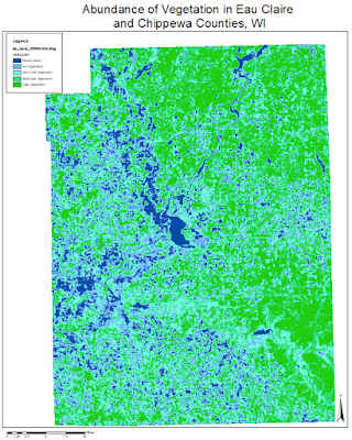
Part two was divided into two parts. The first of which is creating a vegetation health monitoring map using simple band ratio in Erdas Imagine by implementing the normalized difference vegetation index (NDVI). I used the image ec_cpw_2000 for my analysis, this covers Eau Claire and Chippewa counties. I started by imputing my image into Erdas Imagine and then using the raster tool NDVI in the unsupervised category to perform this task. Once the Indices dialog was open I saved the image into the appropriate folder and made sure the sensor was set to Landsat 7 Multispectral, the function as NDVI, and then hit run. I then uploaded the new image into ArcMap and adjusted the symbology to create a map displaying the abundance of vegetation in Eau Claire and Chippewa counties, Wisconsin (Figure 14).

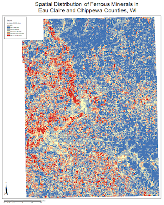
The second section of this lab was mapping the soil health of Eau Claire and Chippewa counties. I did this by performing a band ratio using the ferrous mineral ratio on the image ec_cpw_2000. Once the image was uploaded in Erdas Imagine, I used the Unsupervised raster tool of Indices. In the Indices interface I made sure to save the new image into an appropriate folder, change the sensor to Landsat 7 Multispectral, set the function to Ferrous Minerals, and hit run. Again, I uploaded the new image to ArcMap and created a map to display the spatial distribution of ferrous minerals within Eau Claire and Chippewas counties, Wisconsin (Figure 15).

Results

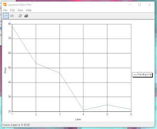Figure 1. Spectral signature of standing water.

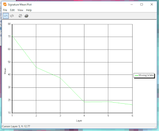Figure 2. Spectral signature of moving water.

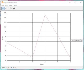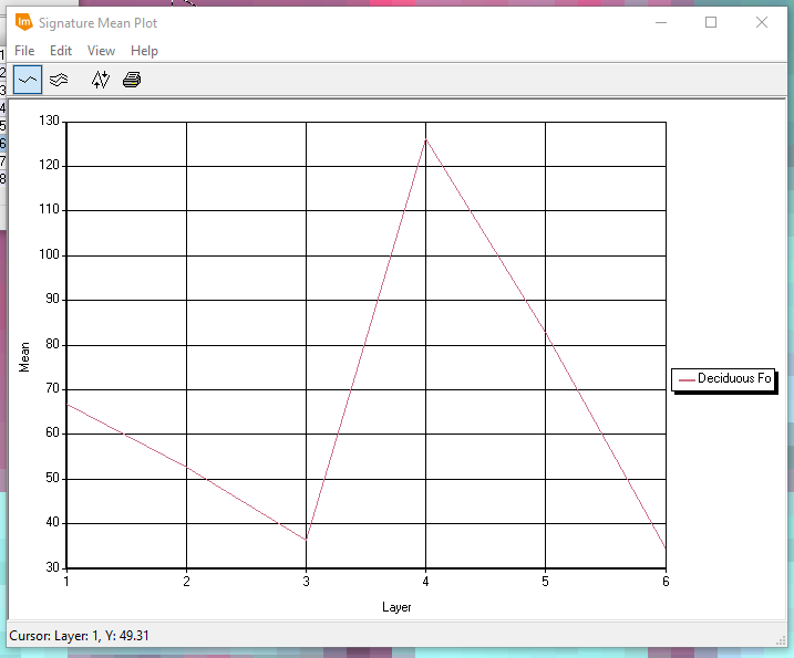
Figure 3. Spectral signature of deciduous forest.

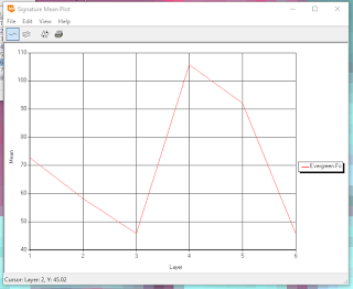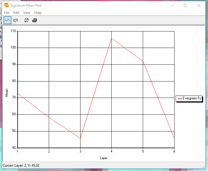
Figure 4. Spectral signature of evergreen forest.

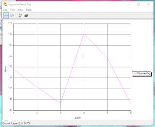Figure 5. Spectral signature of riparian vegetation.

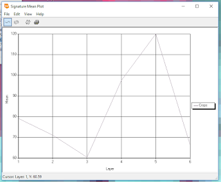Figure 6. Spectral signature of crops.

Figure 7. Spectral signature of dry soil.

Figure 8. Spectral signature of moist soil.

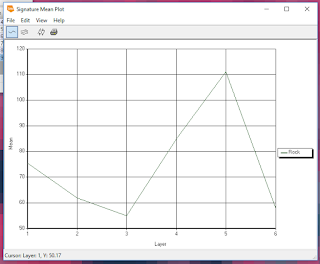Figure 9. Spectral signature of rock.

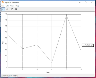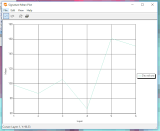
Figure 10. Spectral signature of asphalt highway.

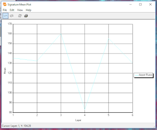Figure 11. Spectral signature of an airport runway.

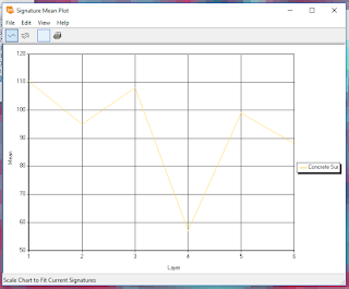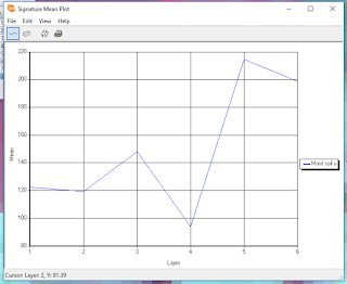
Figure 12. Spectral signature of a concrete surface.

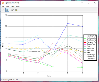Figure 13. All of the above spectral signatures together. As I analyzed this Figure, I noticed many similarities between various signatures. The spectral signatures of standing and moving water are very similar, which is expected due to the fact that the only changing factor is the velocity of the water. The next similar cluster is the vegetation signatures (evergreen forest, deciduous forest, and riparian vegetation). I also expected these to be similar because all plants need to absorb the visible to produce chlorophyll and reflect the NIR in order to avoid damage. The moist and dry soils were also similar, which the exception of the peak in the moist soil in the MIR.